Room Prices Analysis (Part 3): Natural Language Modeling and Feature Selection in Python.
After looking on how to scrape data, clean it and extract geographical information, we are ready to begin the modeling stage.
- Read the Vancouver Room Prices article
- Part 1: Scraping Websites with Python and Scrapy
- Part 2: Data Cleaning and Geolocation with Python and Shapely
In the modeling stage we work to get the answers we need or to build the actual product. For the room prices analysis we are mostly interested in which variables are correlated with high prices so that we can have a better understanding of the market. In other words we want, given the data, to make inferences about the underlying process that generated it.
Alternatively we may also be interested in predicting future prices. The method choice is going to be dependent on the question we want to answer.
Exploratory data analysis
First of all we’re going to do some exploration. The first step is to load the (cleaned) data into our favorite tool, pandas.
Each entry in our dataset corresponds to a post scraped, the data is stored in json format and contains a series of columns with various features. A good thing to do is to use the method DataFrame.head() or to check the attribute DataFrame.columns. The following table represents a subset of the cleaned data (the rest is omitted for brevity), followed by the full list of columns.
| title | latitude | longitude | cats | neigh | updated_on | |
|---|---|---|---|---|---|---|
| 1 | furnished room for rent available april 1 m... | 49.264521 | -123.098803 | NaN | Mount Pleasant | 2015-03-05 11:34:56 |
| 10 | looking for 2 students apr 1 | 49.281699 | -123.133284 | NaN | West End | 2015-03-11 19:37:59 |
| 100 | nice cosy room one block from the beach k... | 49.270175 | -123.167798 | NaN | Kitsilano | 2015-03-04 11:21:14 |
| 1000 | furnished room bathroom in a 2 bed 2bath yal... | 49.275445 | -123.124949 | NaN | Downtown | 2015-03-05 23:43:24 |
| 10000 | 1 bedroom in 2 bedroom condo for rent | 49.264817 | -123.156555 | NaN | Kitsilano | 2015-02-28 13:25:08 |
>>> van_data.columns

Index([u'available_on', u'bedrooms', u'cats', u'city', u'condo', u'content', u'dogs', u'furnished', u'house', u'latitude', u'laundry', u'location', u'longitude', u'neigh', u'parsed_on', u'post_id', u'price', u'size_ft2', u'title', u'updated_on'], dtype='object')
As we can see there is quite a bit of predictors, therefore we may want to run some summaries to check what’s going on. This is done by DataFrame.describe() that will display general statistics for the numerical variables. As you can see some of the predictors are present only for very few posts furnished counts only 21 posts, while the condo variable is not useful as its count is zero.
| bedrooms | cats | condo | dogs | furnished | house | latitude | laundry | longitude | price | size_ft2 | |
|---|---|---|---|---|---|---|---|---|---|---|---|
| count | 92.000000 | 1014 | 0 | 1027 | 21 | 19 | 15013.000000 | 18276 | 15013.000000 | 15438.000000 | 5089.000000 |
| mean | 1.010870 | 1 | NaN | 1 | 1 | 1 | 49.257344 | 1 | -123.093584 | 654.075657 | 869.664767 |
| std | 0.791362 | 0 | NaN | 0 | 0 | 0 | 0.071436 | 0 | 0.509354 | 189.294457 | 4101.154188 |
| min | 0.000000 | 1 | NaN | 1 | 1 | 1 | 43.652228 | 1 | -124.520477 | 300.000000 | 1.000000 |
| 25% | 1.000000 | 1 | NaN | 1 | 1 | 1 | 49.240830 | 1 | -123.132071 | 500.000000 | 189.000000 |
| 50% | 1.000000 | 1 | NaN | 1 | 1 | 1 | 49.261026 | 1 | -123.108394 | 600.000000 | 740.000000 |
| 75% | 1.000000 | 1 | NaN | 1 | 1 | 1 | 49.278292 | 1 | -123.063698 | 750.000000 | 1000.000000 |
| max | 4.000000 | 1 | NaN | 1 | 1 | 1 | 49.823690 | 1 | -79.380315 | 1500.000000 | 145085.000000 |
Now that we have a feel about the quantities we’re dealing with, we want to start exploring the data graphically. Plots are pretty much the best way you have to capture the nature and relationship between variables. In the following plot we use an histogram to display the distribution of the variable price.
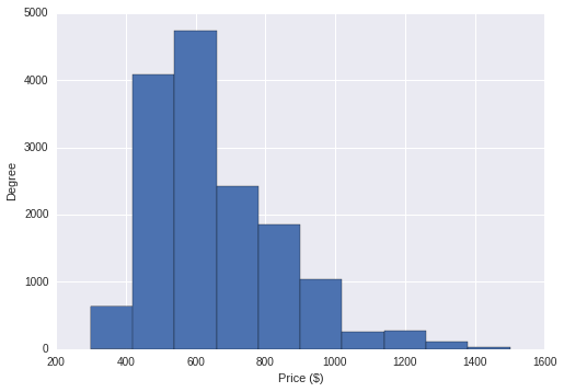
In this case the distribution is quite skewed with a tail at high prices, and a median of about $600. While this is already a great deal of information, we can definitely dig deeper and investigate how price is affected by other measurements.
While histograms and density plots are very informative for single variables, boxplots let us compare several distributions at a glance. The following code groups the price by neighbourhood and displays a boxplot graph. The little rectangles in the boxplots span a range between the first and third quartile (50% of the data) and the vertical line inside of each rectangle is the median, the additional lines (whiskers) are set at a distance of 1.5 times the interquartile range.
van_data.boxplot('price', by='neigh', figsize=(15, 10), rot=90)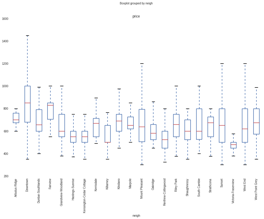
While boxplots can’t tell us how the distribution looks like, they’re still useful to look at the spread and skewness of the distributions. For example, we can see how price varies sensibly with the neighbourhood, and how some neighbourhoods have a much larger price range than others.
Simple natural language modeling, the bag-of-words
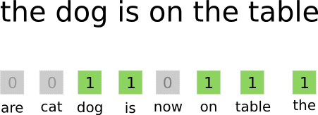
While we got some sparse features from the postings we still have access to a great deal of information: the content of the postings. Understanding natural language (and unstructured data in general) is quite a challenge but, at least for our purposes, it can be effectively addressed with a simple yet popular method, the bag of words.
The idea is to transform the posting text in a vector where each element represent a word. If the word is present, the vector element is set to 1, otherwise it is set to 0.
An even better approach (and the one I used) is to employ bigrams, that is to take into account pairs of words instead of single words. For example the sentence.
python is a dynamic language
Would produce the following bigrams:
python isis aa dynamicdynamic language
Additionally, it is good practice to remove the so called stop words — words that are very frequent but carry very little specific information, for example the, is, it etc.
This bag-of-digrams operation can be easily accomplished with the library scikit-learn as follows. CountVectorizer takes the following arguments:
token_pattern: a regular expression that identifies each word, in this case I excluded numbers.ngram_range: which n-grams to produce, in this case we want 1 and 2-gramsstop_words: remove stop words for the English languagebinary: tellsCountVectorizerto output 1 if the word is in the document 0 otherwise, otherwise it would output a value equals to the number of times the word appears.
The method fit_transform will return the vectorized representation of the content of each post.
# Transform data so that we have no NaN
content_price = van_data[['content', 'price']].dropna()

from sklearn.feature_extraction.text import CountVectorizer
count = CountVectorizer(token_pattern=u'(?u)\\b[a-zA-Z]{2,}\\b',
                        ngram_range=(1, 2),
                        stop_words='english',
                        binary=True)
X = count.fit_transform(content_price.content)
After transforming our input to a bag-of-word (actually a bag of bigrams) representation, we have acquired an enormous amount of features (one for each word in the vocabulary). However, most of those features are very sparse and of little use.
High dimensionality is a big problem and many methods fail or become ineffective when there are a lot of dimensions (see curse of dimensionality), We’ll use some techniques to select the best, most-relevant features.
Feature selection
To think that every single word is important for the price of a room would be naive. Of all those features only few of them have an effect on the price, to extract the important features there are a variety of approaches, I personally prefer the simple ones.
A very simple approach to identify the most relevant features is to run a linear regression using one predictor at a time and to pick only the features that have a (statistically) significant effect on the price. This is already implemented in the package scikit-learn by using the class SelectKBest. The arguments are:
score_func: A score function that tells us how good is the parameter (in this case, it’s the F score of a regression.)k: the number of features to select
In the following code we select the first 200 features that have the biggest effect for the variable price.
from sklearn.feature_selection import SelectKBest, f_regression
kbest = SelectKBest(score_func=lambda x, y: f_regression(x, y, center=False), k=200)
kbest.fit(X, content_price.price)
important = kbest.get_support(True)
Now that we have a more manageable set of candidates we can fine-tune our selection with better methods.
The Lasso
Lasso is one of my favourite techniques, it is similar to a standard linear regression, where we minimize the sum of squares, but instead of minimizing only the sum of squares, we also add a term to prevent the regression coefficients from assuming extreme values and overfit the data. This process is also called as regularization.
Introducing this extra feat is done by adding an extra term to minimize. In particular, we want that the absolute values of the coefficients stays small:
Where:
is the usual sum-of-squares;
is the sum of the absolute values of the coefficients and is a term chosen by the user that controls how much the coefficients are allowed to grow.
One important caveat of the lasso is that the minimization is able to shrink some coefficients to exactly zero, effectively acting as a filter or variable selection method.
The only problem left is picking a good value for . Such parameter optimization is usually handled by a procedure called cross validation.
Cross Validation
Our objective is to pick a value of that eliminates the useless features and produces the best model possible. But what is the best model possible? It’s a model that is more accurate to predict tomorrow’s, or unseen, data.
Cross validation helps producing some unseen data from the data we already have.
We can split the data in 3 (or more generally k) sets, create the model using the first two sets and we optimize the parameter on the third one. Also, we do the same procedure by selecting each time different sets. A figure illustrates the concept better:
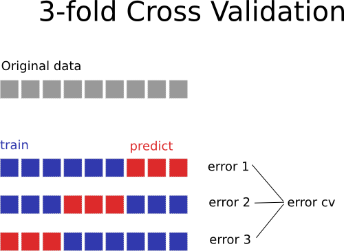
This procedure can give us an estimate of the error we may get on unseen data and we can use this error to optimize parameters (for example )
The cross-validated Lasso is again conveniently implemented in the library scikit-learn, through the class LassoCV. The following code is going to take quite a long time:
from sklearn.linear_model import LassoCV
lasso = LassoCV(cv=3)
lasso.fit(X[:, important], content_price.price)
After the fit is done we can access the coefficients of the lasso through the attribute lasso.coef_. By looking up words in the CountVectorizer we can retrieve terms along with coefficients, ordered from highest (most positively correlated) to lowest.
for c, i in sorted(zip(lasso.coef_, important), reverse=True):
    print "% 20s  | coef: %.2f" % (count.get_feature_names()[i], c)
Notice how the words location and email are exactly 0. They were effectively filtered
by the lasso.
    contact info  | coef: 83.27
       apartment  | coef: 82.04
         parking  | coef: 71.24
           suite  | coef: 67.44
        bathroom  | coef: 48.54
           great  | coef: 44.49
           fully  | coef: 36.13
         bedroom  | coef: 33.68
             bed  | coef: 31.68
             ubc  | coef: 29.53
            pets  | coef: 24.86
        includes  | coef: 21.18
         private  | coef: 20.80
           floor  | coef: 12.55
         looking  | coef: 12.14
         laundry  | coef: 12.09
       vancouver  | coef: 10.92
     living room  | coef: 10.18
            room  | coef: 9.78
           large  | coef: 8.77
        skytrain  | coef: 6.06
          closet  | coef: 5.75
       available  | coef: 4.58
           quiet  | coef: 2.20
        location  | coef: -0.00
           email  | coef: 0.00
       furnished  | coef: -2.71
           clean  | coef: -4.38
        internet  | coef: -5.98
           month  | coef: -7.30
        downtown  | coef: -9.03
           house  | coef: -10.61
        students  | coef: -12.50
            rent  | coef: -13.28
          street  | coef: -14.14
        included  | coef: -15.17
            walk  | coef: -16.28
           cable  | coef: -19.70
             bus  | coef: -21.83
          living  | coef: -23.42
         contact  | coef: -24.57
           close  | coef: -26.25
         station  | coef: -27.18
       utilities  | coef: -29.06
         student  | coef: -32.03
         smoking  | coef: -33.49
         kitchen  | coef: -37.93
          shared  | coef: -41.05
           share  | coef: -58.98
            info  | coef: -65.55
By analyzing the data we were able to obtain a set of candidate words that correlate with higher or lower price. I think this is an interesting result to look at :).
The Model
Now that we have our hands on the most important features we can construct a simple model. Since we’re interested in inference rather than prediction we want to pick something simple like a linear regression.
For inference we are going to use statsmodels, as it gives a more complete statistical treatment for regression. As you’ve seen before, the Lasso implementation in scikit-learn doesn’t give us any indication on how much should we believe those numbers obtained.
While constructing a model for inference you typically want to know how certain variables affect the outcome in question. A simple linear regression allows us to easily obtaining the effect of some variables excluding (controlling) for others. For example, we can see what the effect of the word apartment, regardless on the neighbourhood.
Here is an example model that calculates the price based on neighbourhood, the presence of the word apartment, and the presence of the word shared:
price = a + b * neighbourhood + c * apartment + d * shared
The model can be implemented using statsmodels as follows. There are quite a few points to notice:
- We need to put all the variables nicely in a dataframe that contains the fields
neigh,apartment,sharedandprice; - We need to specify the model, this is done in satsmodels using a special syntax. The code
price ~ 1 + C(neigh, Treatment("none")) + apartment + sharedspecifies that the variablepricedepends onneigh,apartmentandshared; - The part
C(neigh, Treatment("none"))specifies the coding for the variable neigh. In particular we are asking to usenone(neigh not specified) as our reference level (this will be clear later.)
import statsmodels.formula.api as smf
price = content_price.price
neigh = van_data.ix[content_price.index].neigh.fillna('none').values
apartment = X[:, count.vocabulary_['apartment']].toarray().squeeze()
shared = X[:, count.vocabulary_['shared']].toarray().squeeze()

predictor = pd.DataFrame.from_dict({'neigh': neigh, 'apartment': apartment, 'shared': shared, 'price': price})

model = smf.glm('price ~ 1 + C(neigh, Treatment("none")) + apartment + shared', predictor)
fit = model.fit()
fit.summary()| Dep. Variable: | price | No. Observations: | 15438 |
|---|---|---|---|
| Model: | GLM | Df Residuals: | 15413 |
| Model Family: | Gaussian | Df Model: | 24 |
| Link Function: | identity | Scale: | 28414.9282432 |
| Method: | IRLS | Log-Likelihood: | -1.0105e+05 |
| Date: | Sat, 11 Jul 2015 | Deviance: | 4.3796e+08 |
| Time: | 18:29:12 | Pearson chi2: | 4.38e+08 |
| No. Iterations: | 4 |
| coef | std err | z | P>|z| | [95.0% Conf. Int.] | |
|---|---|---|---|---|---|
| Intercept | 625.7286 | 2.507 | 249.622 | 0.000 | 620.816 630.642 |
| C(neigh, Treatment("none"))[T.Arbutus-Ridge] | 102.5775 | 18.650 | 5.500 | 0.000 | 66.024 139.131 |
| C(neigh, Treatment("none"))[T.Downtown] | 199.0859 | 4.932 | 40.369 | 0.000 | 189.420 208.752 |
| C(neigh, Treatment("none"))[T.Dunbar-Southlands] | 79.4633 | 10.774 | 7.375 | 0.000 | 58.346 100.580 |
| C(neigh, Treatment("none"))[T.Fairview] | 151.1972 | 12.375 | 12.218 | 0.000 | 126.942 175.453 |
| C(neigh, Treatment("none"))[T.Grandview-Woodland] | 11.8131 | 10.386 | 1.137 | 0.255 | -8.544 32.170 |
| C(neigh, Treatment("none"))[T.Hastings-Sunrise] | -59.0837 | 6.653 | -8.880 | 0.000 | -72.124 -46.043 |
| C(neigh, Treatment("none"))[T.Kensington-Cedar Cottage] | -55.0974 | 6.042 | -9.119 | 0.000 | -66.940 -43.255 |
| C(neigh, Treatment("none"))[T.Kerrisdale] | 40.4121 | 12.943 | 3.122 | 0.002 | 15.045 65.779 |
| C(neigh, Treatment("none"))[T.Killarney] | -53.0172 | 18.546 | -2.859 | 0.004 | -89.366 -16.668 |
| C(neigh, Treatment("none"))[T.Kitsilano] | 58.5964 | 7.112 | 8.239 | 0.000 | 44.657 72.535 |
| C(neigh, Treatment("none"))[T.Marpole] | 42.1428 | 12.543 | 3.360 | 0.001 | 17.560 66.726 |
| C(neigh, Treatment("none"))[T.Mount Pleasant] | 27.3563 | 9.514 | 2.875 | 0.004 | 8.708 46.004 |
| C(neigh, Treatment("none"))[T.Oakridge] | -16.4488 | 13.199 | -1.246 | 0.213 | -42.318 9.420 |
| C(neigh, Treatment("none"))[T.Renfrew-Collingwood] | -76.9319 | 5.780 | -13.309 | 0.000 | -88.261 -65.603 |
| C(neigh, Treatment("none"))[T.Riley Park] | 51.4610 | 8.902 | 5.781 | 0.000 | 34.014 68.908 |
| C(neigh, Treatment("none"))[T.Shaughnessy] | -7.7521 | 15.181 | -0.511 | 0.610 | -37.506 22.002 |
| C(neigh, Treatment("none"))[T.South Cambie] | 65.9736 | 14.485 | 4.555 | 0.000 | 37.584 94.363 |
| C(neigh, Treatment("none"))[T.Strathcona] | 25.6578 | 13.717 | 1.871 | 0.061 | -1.226 52.542 |
| C(neigh, Treatment("none"))[T.Sunset] | 28.3662 | 7.723 | 3.673 | 0.000 | 13.230 43.502 |
| C(neigh, Treatment("none"))[T.Victoria-Fraserview] | -118.8976 | 10.413 | -11.419 | 0.000 | -139.306 -98.489 |
| C(neigh, Treatment("none"))[T.West End] | 29.8549 | 5.488 | 5.440 | 0.000 | 19.099 40.611 |
| C(neigh, Treatment("none"))[T.West Point Grey] | 59.6830 | 12.770 | 4.674 | 0.000 | 34.654 84.712 |
| apartment | 57.2537 | 3.745 | 15.289 | 0.000 | 49.914 64.593 |
| shared | -13.6907 | 2.921 | -4.687 | 0.000 | -19.416 -7.965 |
Cool, how do we interpret those numbers?
- intercept: the baseline price, that is the price given that neigh is at reference level (that we specified in the coding), apartment and shared are 0 (the post doesn’t contain those two words).
- T.Downtown: how much we should add to the baseline if the posting is from Downtown.
- apartment: how much the presence of the word apartment affects the price
- shared: how much the the presence of the word shared affects the price
Additionally, all this information comes with 95% confidence intervals, that gives us a range in which the true value is supposed to be. For example, given the baseline, being in Downtown with respect to neighbourhood not specified will give you an increase in price that is between $189.420-$208.752 (with 95% confidence).
Other models
There’s quite a bit of models under the sun, here’s a set of improvements that could be of help:
-
An everybodys’ favorite is Random Forest, that can perform both feature selection and regressions and doesn’t overfit. However, while it gives a better accuracy overall, it doesn’t provide easy inference.
-
ElasticNet can be used in place of Lasso, as it deals better with mutlicollinearity.
-
Bayesian general linear models. While much more computationally intensive, I personally feel more comfortable in communicating Bayesian results.