Visualizing Molecular Orbitals in the IPython Notebook

A molecular orbital is a function that describes an electron in a molecule. Visualizing molecular orbitals helps us understand how the electrons are distributed in the molecule.

In this post, we will learn how to read and visualize molecular orbitals from a quantum chemical calculation, all without leaving the IPython Notebook.

The software stack will be:

• chemlab: For general utilities
• cclib: To parse GAMESS output files
• chemview: To visualize molecular orbitals in the browser

To install the software you can conveniently use the Anaconda scientific python distribution that can be downloaded at the following link: http://continuum.io/downloads

After installing Anaconda you can install the software required by running:

conda install -c http://conda.binstar.org/gabrielelanaro chemlab chemview

Extracting the information from the data files

Molecular orbitals are generally produced as a result of some quantum chemical calculation. Typically they are given to the user in the form of a basis set definition and the molecular orbitals coefficients.

What is a basis set? And which coefficients do we need?

The answer comes straight from Wikipedia

A basis set in theoretical and computational chemistry is a set of functions (called basis functions) which are combined in linear combinations (generally as part of a quantum chemical calculation) to create molecular orbitals.

In other words, a molecular orbital \(f(x, y, z)\) is commonly expressed as a linear combination of basis functions \(b_i(x, y, z)\):

All we need to calculate the molecular orbital is to evaluate the basis functions and combine them using the coefficients.

To extract the basis set specification and the molecular orbital coefficients we can use chemlab (that internally uses cclib). In the following code, we retrieve a test calculation directly from the cclib distribution and we extract:

• the molecule geometry molecule
• the basis set specifcation gbasis
• the coefficients mocoeffs.

from chemlab.io import remotefile
url = "https://raw.githubusercontent.com/cclib/cclib/master/data/GAMESS/basicGAMESS-US2012/water_mp2.out"
df = remotefile(url, "gamess")

molecule = df.read('molecule')
molecule.guess_bonds()

mocoeffs = df.read('mocoeffs')
gbasis = df.read('gbasis')

We won’t go in detail on how the gbasis format is structured, it’s enough to say that it contains the specifications on how to construct the basis functions. The coefficients are given by mocoeffs, which is a list containing a single matrix of shape (7, 7).

print(mocoeffs)

[array([[ 0.994203,  0.025916, -0.      ,  0.003993, -0.      , -0.005627, -0.005627],
        [-0.234218,  0.845882, -0.      ,  0.117048, -0.      ,  0.156449,  0.156449],
        [ 0.      ,  0.      ,  0.603305,  0.      ,  0.      ,  0.446377, -0.446377],
        [ 0.100458, -0.521395, -0.      ,  0.774267, -0.      ,  0.289064,  0.289064],
        [ 0.      ,  0.      ,  0.      ,  0.      ,  1.      ,  0.      ,  0.      ],
        [-0.128351,  0.832526,  0.      ,  0.732626,  0.      , -0.775801, -0.775801],
        [ 0.      ,  0.      ,  0.976485,  0.      ,  0.      , -0.808916,  0.808916]])]

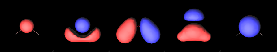
Each row of the matrix corresponds to the set of coefficients for a given molecular orbital (in this case we have a total of 7 molecular orbitals).

Molecular orbitals as functions

Now we want to transform this specification into a standard function that, given a set of \( (x ,y ,z) \) coordinates, returns a value corresponding to the function at that point. This can be accomplished through the chemlab.qc.molecular_orbital function.

In the following snippet we create a function representing the 4th molecular orbital and we evaluate it at (0, 0, 0).

from chemlab.qc import molecular_orbital

coefficients = mocoeffs[0][3] # 4th because we start counting from 0
f = molecular_orbital(molecule.r_array, coefficients, gbasis)
print(f(0, 0, 0))
# 2.67271724871

Now that we have an actual function that outputs real numbers, we can plot it using the chemview library.

Visualizing the molecular orbitals as isosurfaces

One of the most popular ways to visualize a molecular orbital is to plot it as an isosurface. Isosurfaces can give us a feeling of what the shape of the function (or the field) looks like.

Plotting isosurfaces is fairly easy with chemview. We first need to do the necessary imports:

from chemview import enable_notebook, MolecularViewer
enable_notebook()

Next, we want to create a chemview.MolecularViewer instance and to visualize the molecule as a wireframe:

# Initialize molecular viewer
mv = MolecularViewer(molecule.r_array, { 'atom_types': molecule.type_array,
                                         'bonds': molecule.bonds })
mv.wireframe()
mv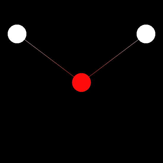

Finally, we render the molecular orbital using the MolecularViewer.add_isosurface method. We render the surface for which the molecular orbital evaluates to 0.3 (positive sign) in blue, and the surface corresponding to an isovalue of -0.3 (negative sign) in red.

mv.add_isosurface(f, isolevel=0.3, color=0xff0000)
mv.add_isosurface(f, isolevel=-0.3, color=0x0000ff)

mv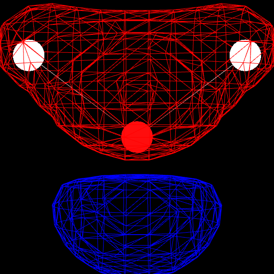

You can now play around with the output, try different orbitals, changing the isovalue, colors and style of the isosurface.

Hopefully that gave you an idea of the outstanding capabilities of IPython notebook and the available chemistry libraries. Not only making your scripts in the notebook can save you a lot of time, but having this level of control and granularity gives you the possiblity to do a kind of analysis which is impossible with the standard black-box tools commonly used by computational chemists.

By the way, if you’re interested in maintaining a quantum chemistry package in chemlab let me know in an email!

Share this Post