3 Feb 2016

Evaluation measures for multiclass problems

In most machine learning courses a lot of emphasis is given to binary classification tasks. However, I found that the most useful machine learning tasks try to predict multiple classes and more often than not those classes are grossly unbalanced.

One example of that was the AirBnB kaggle competition, in which I recently participated with Francesco Pochetti. You can check the produced notebook at this link: https://github.com/FraPochetti/Airbnb/blob/0de547746b6f4cfbe4914ec1a1c4b38077c01c0e/AirbnbKaggleCompetition.ipynb.

Confusion matrix

Given a generic problem, a very useful and intuitive measure is the confusion matrix. It is built from the list of predicted classes versus the true classes. To illustrate this with an example let’s imagine we have a test set with the following labels:

A A A A C C C B B

and our model predicts:

A B A B C C C A B

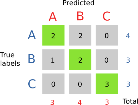
We can see that sometimes instead of predicting A, our model predicts B. We can build a matrix by counting how many times a certain pair occurs. In our case, for example, when the real label is A we predict A for 2 times, B for 2 times and C for 0 times.

By putting the counts for all possible combinations in a table, we obtain the confusion matrix (see below picture). The usefulness of the confusion matrix lies in its interpretability, it is obvious by looking at it where the problem lies with our model. In this case C is predicted perfectly while we got some problems with A.

Sometimes, especially when optimizing model parameters, it is useful to have a single value that summarizes the content of the table. Unfortunately there is no single answer to this question, but one can choose an appropriate metric, depending on the problem at hand.

Precision

Precision is the number of correct prediction divided by the number of total predictions made. Intuitively, a high precision for a class means that if our models predict that class, it is very likely to be true. A high precision model will be useful in those situations where we need to have an high confidence in our prediction (for example in medical diagnosis).

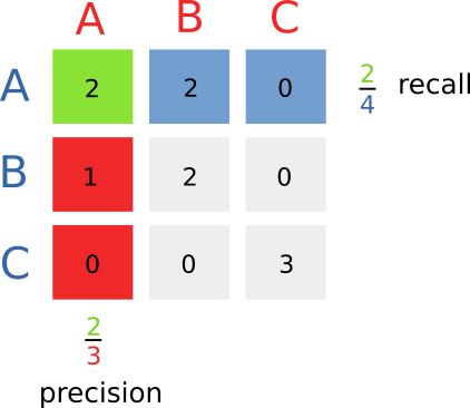
Precision can be calculated separately for each class. Graphically, for each row, we take the number on the diagonal, and divide it by the sum of all the elements in the column.

prec_A = 2/3 = 0.67
prec_B = 2/4 = 0.50
prec_C = 3/3 = 1.00

The drawback of precision is that, if you have a problem where there are 1000 instances of A, if the model predicts gives a single prediction for A, and the prediction is correct, it will have a perfect score of 1. What about the fact that the model failed to detect the other 999 instances of A? The other side of the coin is recall.

Recall

Recall is the number of correct predictions divided by the total number of elements present in that class. Graphically, it is the value on the diagonal, divided by the sum of the values in the row. If recall is high, it means that our models manages to recover most instances of that class. Obtaining high recall is very easy, it’s sufficient to say that everything matches that class, and you can be sure that all the elements are retrieved.

recall_A = 2/4 = 0.50
recall_B = 2/3 = 0.67
recall_C = 3/3 = 1.00

As you can see in the case of C, if we recover all classes, and all our prediction are correct, we obtain a perfect score for both precision and recall.

And now a graphical picture of precision and recall for class A

F1-score

F1 score is the harmonic mean of precision and recall, and acts as a combined measure of the two.

$F_1 = 2 \frac{p \cdot r}{p + r}$

See also $F_\beta$ score to bias the measure more towards precision or recall.

Micro and macro averages

To extract a single number from the class precision, recall or F1-score, it is common to adopt two different kinds of average.

The first, is to compute the score separately for each class and then taking the average value — this is called macro averaging. This kind of averaging is useful when the dataset is unbalanced and we want to put the same emphasis on all the classes.

$\frac {r_A + r_B + r_C}{3} = 0.7233$

The second is to calculate the measure from the grand total of the numerator and denominator, this is called micro averaging and is useful when you want to bias your classes towards the most populated class. For our recall example:

$\frac{2 + 2 + 3}{4 + 3 + 3} = 0.636$

Accuracy

Accuracy is another measure that can be useful when the problem has well balanced classes (for example in optical character recognition) and we want to put an emphasis on exact matches. Unforunately accuracy suffers on unbalanced data sets, a typical example is information retrieval.

Graphically, it is the sum of the element on the diagonal of the confusion matrix divided by the total number of predictions made.

Cross entropy

Sometimes we are not interested in the class predictions, instead, we are trying to model the class probabilities themselves(how probable is each class given the predictors?).

Cross entropy measures how good the predicted probabilities match the given data. This is calculated using the following formula:

$-\sum_{i}^N \sum_j^M y_{ij} \ln p_{ij}$

Where $i$ runs over the number of samples and $j$ runs over the number of classes. By the formula alone this measure is not too easy understand but it is actually fairly simple to compute.

For each sample:

Make a one-hot encoding of the true labels, eg. $y_1 = A = [1, 0, 0]$
Use your model to predict probabilities , eg. $p_1 = [0.7, 0.2, 0.1]$
Take the element-wise product of the label and probability: $y_1 \cdot p_1 = \ln(0.7)$
Do the same for all the other samples and take the negative of the sum

Cross-entropy is often called log-loss, because it can be used as a loss function in logistic regression, or binomial deviance, because it is the deviance of a binomial distribution.

As cross entropy deals with probabilities, it evaluates the overall goodness of model, and it is often used in data science competitions. Being a sum over every data point, this measure is also affected by heavily skewed data sets.

References:

NDCG

Normalized discounted cumulative gain was the measure used in the AirBnB Kaggle competition, this measure is appropriate when dealing with ranked results, as it gives the value of 1 when the best possible rank for the query is achieved.

To get back to our previous 3 class example, instead of making a prediction, we could rank the samples. If the real label is “A”, all those ranks are equally good:

A B C
A C B
A A A

While the rank B A C would be better than B C A, because the correct label is higher in the position. To calculate this quantity in this specific case (where there is a single relevant result in our set), it is sufficient to apply the formula:

$\frac{1}{\log_2 (r)}$

where r is the position of the correct answer in our prediction. You can see how the higher the rank is, the lower the score becomes. After doing that, it is necessary to take the average of the NDCG score for every prediction.

What I’ve written is a gross semplification, the actual definition of NDCG is more general and you can learn more about it on https://en.wikipedia.org/wiki/Discounted_cumulative_gain.

Tips for dealing with unbalanced datasets

Unbalanced datasets are really common to come across, so first of all make sure to explore your confusion matrix to verify that your models are producing results that are non-trivial (like predicting all he time the most represented class). Picking the wrong measure is like answering the wrong question:

How is the weather? I’m going to the movies.

Some models are really good at dealing with unbalanced data sets. For example ensemble methods (Boosted regression trees, random forest etc.) allow you to assign a weight to the samples, by using a weight that is the inverse frequency of the class population, you can “boost” the influence of the least represented classes.

Models like SVM instead, suffer more from this aspect, but if you have to, you can still use oversampling of the least frequent classes and subsampling of the most frequent ones.